
Bearing Modeling · Engineering Software
BearingSolver: Physics-Based Bearing Analysis
Scilab engineering tool for deep-groove ball bearing sizing, combining traceable physics models, a reusable GUI, and validated outputs in under three seconds.
VALIDATED
Role
R&D Engineer
Company
Involute Transmissions - France
Period
May 2025 – September 2025
Problem
Early bearing-sizing studies required repeated calculations of life, operating clearance, stiffness, contact pressure, and frictional losses across multiple operating conditions. A complete manual analysis could take approximately 5–10 hours and had to be repeated whenever the bearing geometry, material, fit, temperature, lubrication, or loading changed.
Commercial tools reduced calculation time but introduced license costs, complex workflows, and limited visibility into their equations, assumptions, and accuracy. Involute Transmissions therefore needed an internal engineering application that was fast and easy to use while keeping every model traceable and its validation margin known.
Core requirements
- Calculate bearing life, operating clearance, radial and axial response, contact pressure, frictional losses, and lubrication indicators.
- Support multiple operating cases with axial, radial, and combined loads and prescribed misalignment.
- Provide a Scilab GUI with study-file management, input checks, contextual help, and model-validity warnings.
- Document every equation, assumption, symbol, applicability limit, and known model boundary.
- Validate the implemented models against standards, literature, commercial software, and available physical-test evidence.
Solution
I developed BearingSolver as a modular Scilab application that consolidates the complete deep-groove ball bearing analysis workflow into one traceable engineering interface. Engineers can define bearing geometry and materials, create multiple operating cases, run the implemented models, compare performance, and save studies for later reuse.
The computational core combines documented bearing theory, standards-based calculations, and nonlinear numerical solving. Each result remains connected to known equations, assumptions, applicability limits, and validation evidence. Input controls, contextual help, detailed result views, and model-validity warnings help engineers interpret the outputs rather than treating every calculated value as automatically trustworthy.
Platform capabilities
- Study-file creation, saving, reopening, and comparison.
- Bearing geometry, material, fit, temperature, lubrication, and multi-case load definition.
- Life, damage, operating-clearance, viscosity-ratio, deformation, stiffness, contact-pressure, and frictional-loss calculations.
- Result tables, load-distribution charts, contact-surface views, and operating-case comparisons.
- Input verification, contextual help, detailed calculation views, and model-validity warnings.
Method
Step 1 — Establish the modeling foundation
Before programming, I identified the physical phenomena and outputs that BearingSolver had to model. I then conducted a structured literature review using SKF technical resources, British Gear Association training, the Harris bearing-analysis references, ISO 281:2007, and relevant scientific publications.
For each candidate model, I documented its required inputs, calculated outputs, assumptions, applicability limits, and available validation references. This established a traceable calculation chain covering bearing geometry, operating clearance, Hertzian contact behavior, load distribution, deformation, stiffness, life, lubrication indicators, and frictional losses. The resulting 65-page technical note became the implementation specification for the computational models.

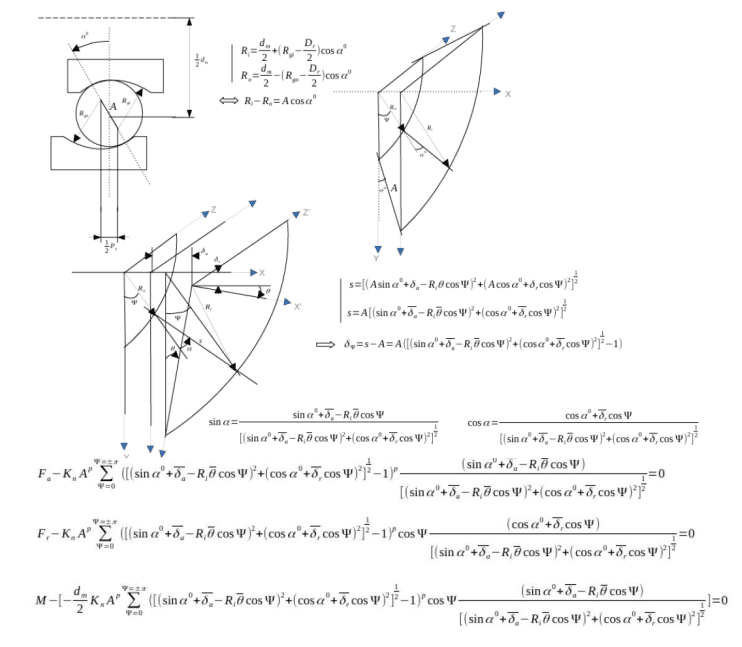
- Defined the calculation chain from bearing geometry and operating conditions to mechanical performance.
- Selected generalized Hertzian theory for contact behavior and ISO 281:2007 for bearing-life calculations.
- Documented each model's inputs, outputs, assumptions, equations, and applicability limits.
- Converted known model boundaries into requirements for software checks and user warnings.
Step 2 — Translate theory into computational models
I converted the selected physical models into modular Scilab functions, progressing from bearing geometry and operating clearance to Hertzian contact, radial and axial response, combined loading, life, and frictional losses. Each function used defined engineering inputs and returned traceable outputs that could be reused by the interface and tested independently during validation.
Radial equilibrium was solved iteratively by adjusting bearing displacement until the forces generated by the loaded rolling elements balanced the applied load. Axial response used the Jones stiffness formulation and Scilab's nonlinear solver to determine contact angle and deformation. Combined loading required a coupled three-equation equilibrium system for axial, radial, and angular behavior.
I reformulated the coordinate system to make the internal kinematics easier to interpret and used prescribed misalignment as a practical engineering input. When the advanced ISO fatigue-limit formulation did not converge reliably, I retained the documented simplified method instead of delivering an unstable solver. The excluded capability and its consequences remained visible in the model documentation and interface warnings.
- Implemented modular functions for clearance, contact, deformation, stiffness, life, and frictional losses.
- Used iterative equilibrium and nonlinear numerical solving for radial, axial, and combined-load response.
- Standardized model inputs and outputs for reuse by the GUI and independent validation.
- Documented numerical simplifications and exposed their applicability limits to users.
Step 3 — Build the Engineering GUI
I transformed the computational models into a Scilab GUI organized around the engineer’s complete analysis sequence: define the bearing geometry and materials, create multiple operating cases, execute the calculations, inspect the results, and explore the detailed contact behavior.
Every field, control, and result panel was programmed and connected to the underlying calculation functions. The interface presents load distribution, deformation, stiffness, contact pressure, and validity information through structured tables and plots. Contextual help, input checks, and explicit warnings—such as identifying truncated contact surfaces—help users distinguish a numerical result from one that is valid for engineering use.
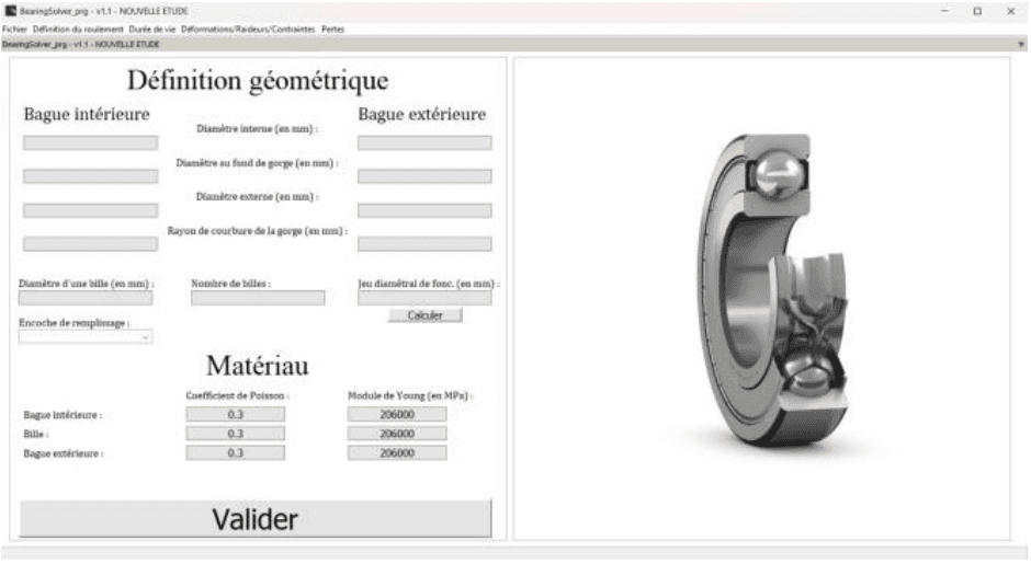
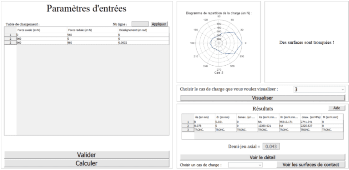
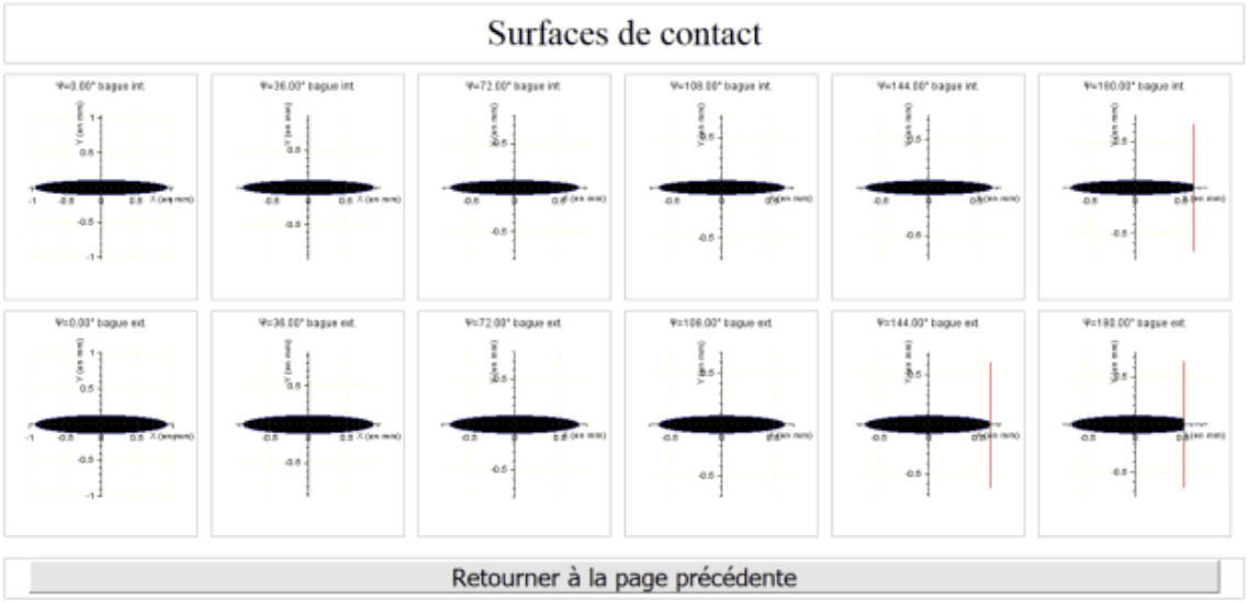
- Structured the application around bearing definition, operating cases, calculation, and result review.
- Connected standardized GUI inputs and outputs to the modular Scilab models.
- Visualized load distribution, mechanical results, and individual contact surfaces.
- Integrated input checks, contextual help, detailed views, and model-validity warnings.
- Enabled study files to be saved and reopened for repeatable analysis.
Step 4 — Validate the Models and Quantify Their Precision
I validated BearingSolver through a progressive chain of independent evidence. I first benchmarked the implemented calculations against SKF SimPro, then cross-checked their physical behavior and reference cases against NASA technical publications, Harris bearing-analysis examples, and the ISO 281 bearing-life standard. The final stage compared the model predictions with the available evidence from the company’s bearing test-bench process.
The test-bench results were not used to calibrate or correct the computational models. Instead, I recorded every validation test, its reference conditions, its results, and the observed differences in a 200-page validation note covering the complete campaign. This body of evidence allowed me to quantify the precision of each model and make its expected accuracy traceable to the engineering team. A separate user guide documented the complete application workflow.

- Benchmarked the implemented calculations against SKF SimPro commercial software.
- Cross-checked model behavior with NASA publications, Harris examples, and ISO 281.
- Compared model predictions with the available company test-bench evidence.
- Recorded every validation test, reference result, and observed difference in a 200-page validation note.
- Used the measured differences to define the precision of each model without calibrating it against the test-bench results.
Results
BearingSolver was delivered as a reusable internal Scilab application for deep-groove ball bearing analysis. Calculations that could require approximately 5–10 hours when performed manually were reduced to around 20 ms for selected models, while the complete result set could be generated in under three seconds. Each model’s precision was established through documented comparisons rather than test-bench calibration.
Delivered outcomes
Complete engineering workflow
- Life, damage, clearance, deformation, stiffness, contact-pressure, and frictional-loss calculations.
- Axial, radial, and combined loading with prescribed misalignment.
- Multi-case studies, detailed results, load-distribution plots, and contact-surface visualization.
Calculation time reduced
- Selected calculations reduced from approximately 5–10 hours of manual work to around 20 ms.
- Complete application outputs generated in under three seconds.
- Study files made analyses repeatable and easier to compare.
Precision and traceability documented
- Predictions compared with SKF SimPro, NASA publications, Harris references, ISO 281, and available test-bench results.
- Model precision defined from the observed differences and recorded in a 200-page validation note.
- Modeling theory documented in a 65-page technical note, with a separate user guide for engineering reuse.